Ionisation: the measured yields of N2 and O2

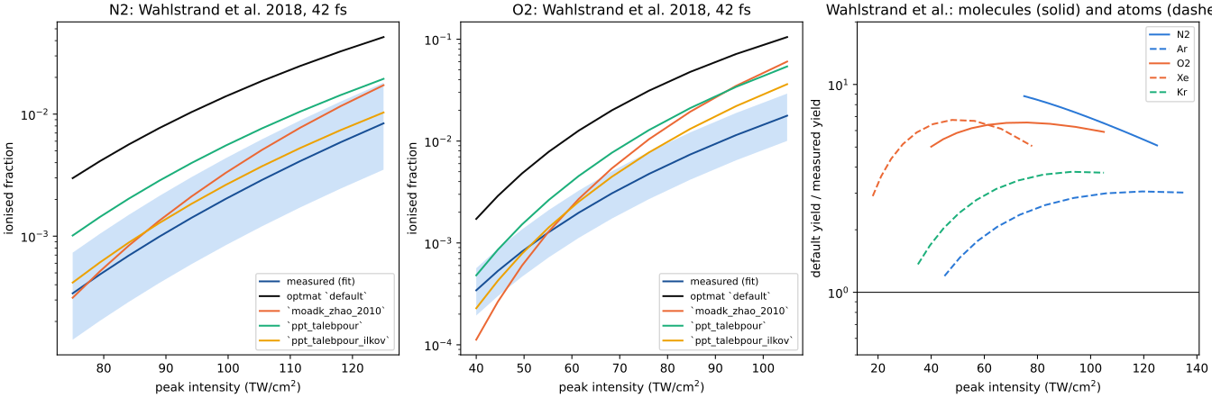
Wahlstrand et al. (2018) measured the absolute yield of N2 and O2 in the same experiment as that of argon, krypton and xenon: 800 nm, 42 fs, the electron density from the refractive index of the plasma, at a local intensity calibrated through the Kerr effect to 13 %.

Left and centre: the measurement (the fit of the Supplemental Material) with the band of its intensity’s uncertainty, and the yields of the default model and of the literature’s forms, of one electron, on the envelope of the pulse. The default lies 5 to 9 times above N2’s measurement and 5.0 to 6.5 times above O2’s. Of the forms, the effective-charge rate in Ilkov et al.’s form (ppt_talebpour_ilkov) comes closest, although its charges were fitted within the static Coulomb factor (TC-674).

Right: the default’s yield over the measurement, for the molecules and for the atoms of the same experiment. The current atomic defaults give rate-to-measurement ratios of 1.2 to 3.1 (Ar), 1.4 to 3.8 (Kr) and 2.9 to 6.8 (Xe). The atomic electron counts and Coulomb factor affect this comparison; the earlier static-factor comparison is recorded in TC-660, TC-680 and TC-698. See Molecular ionisation: validation and limitations and Noble-gas ionisation: measured yields for the numerical tables and calibration limits.

import warnings

import matplotlib.pyplot as plt
import numpy as np
from _helpers import COLOURS

from optmat.exceptions import ModelRangeWarning
from optmat.gas.ionisation_validation import measured_yields

MODELS = {
    "default": ("optmat `default`", "#0b0b0b"),
    "moadk_zhao_2010": ("`moadk_zhao_2010`", COLOURS[1]),
    "ppt_talebpour": ("`ppt_talebpour`", COLOURS[2]),
    "ppt_talebpour_ilkov": ("`ppt_talebpour_ilkov`", COLOURS[3]),
}
INTENSITY_UNCERTAINTY = 0.13  # Wahlstrand et al. 2018, caption of Fig. 3

fig, axes = plt.subplots(1, 3, figsize=(14, 4.6), layout="constrained")
with warnings.catch_warnings():
    # The forms without a correction are drawn beyond the barrier-suppression field.
    warnings.simplefilter("ignore", ModelRangeWarning)
    for axis, gas in zip(axes[:2], ("N2", "O2"), strict=True):
        measured = measured_yields(gas)
        x = measured.x / 1e16
        power = np.log(measured.expected[-1] / measured.expected[0]) / np.log(
            x[-1] / x[0]
        )
        axis.fill_between(
            x,
            measured.expected * (1 - INTENSITY_UNCERTAINTY) ** power,
            measured.expected * (1 + INTENSITY_UNCERTAINTY) ** power,
            color="#86b6ef",
            alpha=0.4,
            lw=0,
        )
        axis.semilogy(x, measured.expected, color="#184f95", label="measured (fit)")
        for name, (label, colour) in MODELS.items():
            comparison = measured_yields(gas, name)
            axis.semilogy(x, comparison.predicted, color=colour, label=label)
        axis.set_xlabel("peak intensity (TW/cm$^2$)")
        axis.set_ylabel("ionised fraction")
        axis.set_title(f"{gas}: Wahlstrand et al. 2018, 42 fs")
        axis.legend(fontsize=8, loc="lower right")

    for colour, (molecule, atom) in zip(
        COLOURS, (("N2", "Ar"), ("O2", "Xe")), strict=False
    ):
        for gas, style in ((molecule, "-"), (atom, "--")):
            comparison = measured_yields(gas)
            axes[2].semilogy(
                comparison.x / 1e16,
                comparison.ratio,
                color=colour,
                ls=style,
                label=gas,
            )
    kr = measured_yields("Kr")
    axes[2].semilogy(kr.x / 1e16, kr.ratio, color=COLOURS[2], ls="--", label="Kr")
axes[2].axhline(1.0, color="#0b0b0b", lw=0.8)
axes[2].set_ylim(0.5, 20)
axes[2].set_xlabel("peak intensity (TW/cm$^2$)")
axes[2].set_ylabel("default yield / measured yield")
axes[2].set_title("Wahlstrand et al.: molecules (solid) and atoms (dashed)")
axes[2].legend(fontsize=8)
plt.show()