Fused silica: the complex index and n2

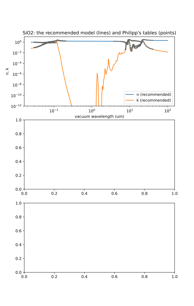
Top: the recommended model’s n and k (fit/SiO2: Franta et al.’s universal dispersion model of Lithosil Q2 refitted to the absolute refractometry of the window, TC-399) from 25 nm to 100 um. The points are Philipp’s tables in Palik’s handbook (philipp_1985); only Hunter’s and the Philipp-Lamy EUV points are close to Franta’s measurement-based model, as TC-324 records.

Middle: the transparent window, as differences in n from the recommended model: Leviton & Frey’s absolute formula at 20 degrees C, Malitson’s formula taken from room air to vacuum, Arosa’s as published (relative to air), Franta’s published model, and Malitson’s three prisms (points).

Bottom: n2 against wavelength, the fitted long-pulse n2 (band: one sigma) and its electronic part, with each source’s values scaled by the fit’s calibration factor (kerr/SiO2, TC-393).

import matplotlib.pyplot as plt
import numpy as np

from optmat.datasets import datasets
from optmat.solid.kerr import kerr_models, load_config, points
from optmat.solid.models.formulas import FormulaModel
from optmat.solid.models.registry import default_model, models

silica = default_model("SiO2")
wavelength = np.geomspace(25e-9, 100e-6, 3000)
index = silica.refractive_index(wavelength)

fig, (top, middle, bottom) = plt.subplots(3, 1, figsize=(7, 11))
top.loglog(wavelength * 1e6, np.real(index), label="n (recommended)")
top.loglog(wavelength * 1e6, np.imag(index), label="k (recommended)")
for dataset in datasets("SiO2"):
    if dataset.source != "philipp_1985" or dataset.use == "reproduced":
        continue
    x = dataset.vacuum_wavelength() * 1e6
    marker = "o" if dataset.quantity == "refractive_index" else "s"
    if dataset.quantity in {"refractive_index", "extinction_coefficient"}:
        top.loglog(x, dataset.scaled_values(), marker, ms=2, color="0.4")
top.set_ylim(1e-12, 10)
top.set_xlabel("vacuum wavelength (um)")
top.set_ylabel("n, k")
top.set_title("SiO2: the recommended model (lines) and Philipp's tables (points)")
top.legend()

<matplotlib.legend.Legend object at 0x76db1a0f5fd0>

window = np.linspace(0.22e-6, 3.7e-6, 400)
reference = np.real(silica.refractive_index(window))
for name in (
    "leviton_2008/sellmeier",
    "malitson_1965/sellmeier",
    "arosa_2020/sellmeier_fit3",
    "franta_2016/udm_lithosil_q2",
):
    model = models("SiO2")[name]
    if isinstance(model, FormulaModel) and model.temperature is not None:
        model = model.at_temperature(293.15)
    low, high = model.wavelength_range
    inside = (window >= low) & (window <= high)
    difference = np.real(model.refractive_index(window[inside])) - reference[inside]
    middle.plot(window[inside] * 1e6, difference * 1e4, label=name)
for dataset in datasets("SiO2", quantity="refractive_index_deviation"):
    if not dataset.id.startswith("residual_") or dataset.use != "primary":
        continue
    x = dataset.vacuum_wavelength()
    malitson = models("SiO2")["malitson_1965/sellmeier"]
    measured = dataset.scaled_values() + np.real(malitson.refractive_index(x))
    shown = measured - np.real(silica.refractive_index(x))
    middle.plot(x * 1e6, shown * 1e4, ".", ms=3, color="0.4")
middle.axhline(0, color="k", lw=0.5)
middle.set_xlabel("vacuum wavelength (um)")
middle.set_ylabel("n - n(recommended)  (1e-4)")
middle.set_title("The transparent window: the published models and Malitson's prisms")
middle.legend(fontsize="small")

<matplotlib.legend.Legend object at 0x76db18e79fd0>

kerr = kerr_models()["kerr/SiO2"]
grid = np.linspace(0.36e-6, 3.4e-6, 200)
n2 = kerr.n2(grid) * 1e20
sigma = kerr.n2_sigma(grid) * 1e20
bottom.fill_between(grid * 1e6, n2 - sigma, n2 + sigma, alpha=0.3)
bottom.plot(grid * 1e6, n2, label="n2 (long pulse)")
bottom.plot(grid * 1e6, kerr.n2_electronic(grid) * 1e20, "--", label="electronic part")
for options in load_config("SiO2").fitted:
    values = points(options)
    scale = kerr.scales[options.group]
    bottom.plot(values.wavelength * 1e6, values.value / scale * 1e20, ".", color="0.4")
bottom.set_xlabel("vacuum wavelength (um)")
bottom.set_ylabel("n2 (1e-20 m^2/W)")
bottom.set_title("n2: the fit and the data (each source divided by its scale)")
bottom.legend()
fig.tight_layout()
plt.show()