Dispersion uncertainty and sensitivity to dataset selection

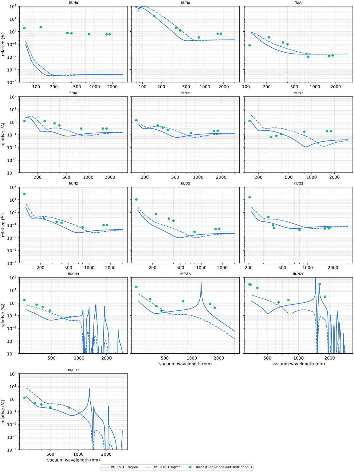
How well each fitted model knows the group-velocity dispersion \(\beta_2\) and the third-order dispersion \(\beta_3\): the relative one-sigma uncertainty propagated from the fit’s covariance (scaled by the reduced chi-squared where it exceeds one; dispersion_sigma_relative()), against wavelength over each model’s range. In the dilute limit these relative uncertainties do not depend on pressure or temperature.

The points are the empirical check: the largest change of \(\beta_2\) when one dataset is left out of the fit (tools/fit/robustness.py). Where they lie well above the solid line, the fit is sensitive to that dataset beyond its statistical uncertainty. This sensitivity does not include all possible systematic errors.

The printed table gives statistical uncertainties at 800 nm; the manual chapter Gas dispersion: accuracy and limitations discusses how to interpret them.

The uncertainties are statistical: they do not include the choice of model form or the unresolved disagreements between sources (TC-92, TC-95, TC-101).

gas   GVD 1 sigma  TOD 1 sigma
He        0.0004%      0.0004%
Ne        0.2091%      0.1852%
Ar        0.0162%      0.0177%
Kr        0.1067%      0.0863%
Xe        0.0899%      0.0672%
N2        0.0116%      0.0860%
H2        0.0267%      0.0519%
D2        0.0161%      0.0103%
O2        0.0555%      0.0905%
CH4       0.0756%      0.0412%
SF6       0.2705%      0.1223%
N2O       0.6628%      0.1428%
CO2       0.0538%      0.2198%

import json

import matplotlib.pyplot as plt
import numpy as np

from optmat.gas import GAS_DATA_DIRECTORY
from optmat.gas.fitting import HARTREE_NM
from optmat.gas.models.fitted import fitted_models

GASES = [
    *("He", "Ne", "Ar", "Kr", "Xe"),
    *("N2", "H2", "D2", "O2", "CH4", "SF6", "N2O", "CO2"),
]
fits = fitted_models()

print(f"{'gas':4s} {'GVD 1 sigma':>12s} {'TOD 1 sigma':>12s}")
fig, axes = plt.subplots(5, 3, figsize=(12, 16), layout="constrained", sharey=True)
for ax in axes.flat[len(GASES) :]:
    ax.set_visible(False)
for ax, gas in zip(axes.flat, GASES, strict=False):
    fit = fits[f"fit/{gas}"]
    longest = min(3e-6, 0.999 * fit.wavelength_range[1])  # below any infrared pole
    grid = np.geomspace(1.1 * fit.wavelength_range[0], longest, 300)
    omega = HARTREE_NM / (grid * 1e9)
    gvd = fit.dispersion_sigma_relative(omega, 2) * 100
    tod = fit.dispersion_sigma_relative(omega, 3) * 100
    ax.plot(grid * 1e9, gvd, color="#2a78d6", label="fit: GVD 1 sigma")
    ax.plot(grid * 1e9, tod, color="#2a78d6", linestyle="--", label="fit: TOD 1 sigma")
    record = json.loads(
        (GAS_DATA_DIRECTORY / "models" / "robustness" / f"{gas}.json").read_text(
            encoding="utf-8"
        )
    )
    largest = np.max(
        [np.abs(entry["gvd_shift_relative"]) for entry in record["dropped"].values()],
        axis=0,
    )
    ax.plot(
        record["wavelength_nm"],
        largest * 100,
        "o",
        color="#1baf7a",
        ms=5,
        label="largest leave-one-out shift of GVD",
    )
    at_800 = HARTREE_NM / np.array([800.0])
    print(
        f"{gas:4s} {fit.dispersion_sigma_relative(at_800, 2)[0] * 100:11.4f}% "
        f"{fit.dispersion_sigma_relative(at_800, 3)[0] * 100:11.4f}%"
    )
    ax.set_xscale("log")
    ax.set_yscale("log")
    ax.set_ylim(1e-4, 100)
    ax.set_title(f"fit/{gas}", fontsize=8)
    ax.grid(which="both", alpha=0.25)
    ticks = [t for t in (50, 100, 200, 500, 1000, 2000) if t >= grid[0] * 1e9 / 1.2]
    ax.set_xticks(ticks, [str(t) for t in ticks])
    ax.xaxis.set_minor_formatter(plt.NullFormatter())
handles, labels = axes[0, 0].get_legend_handles_labels()
fig.legend(handles, labels, loc="outside lower center", ncol=4, fontsize=8)
for ax in axes[:, 0]:
    ax.set_ylabel("relative (%)")
for ax in axes.flat[len(GASES) - 3 : len(GASES)]:  # the bottom of each column
    ax.set_xlabel("vacuum wavelength (nm)")
plt.show()