Ionisation: optmat’s rate of molecules

The default rate of molecules (optmat.gas.molecular_ionisation_rates.molecular_rate_model()).

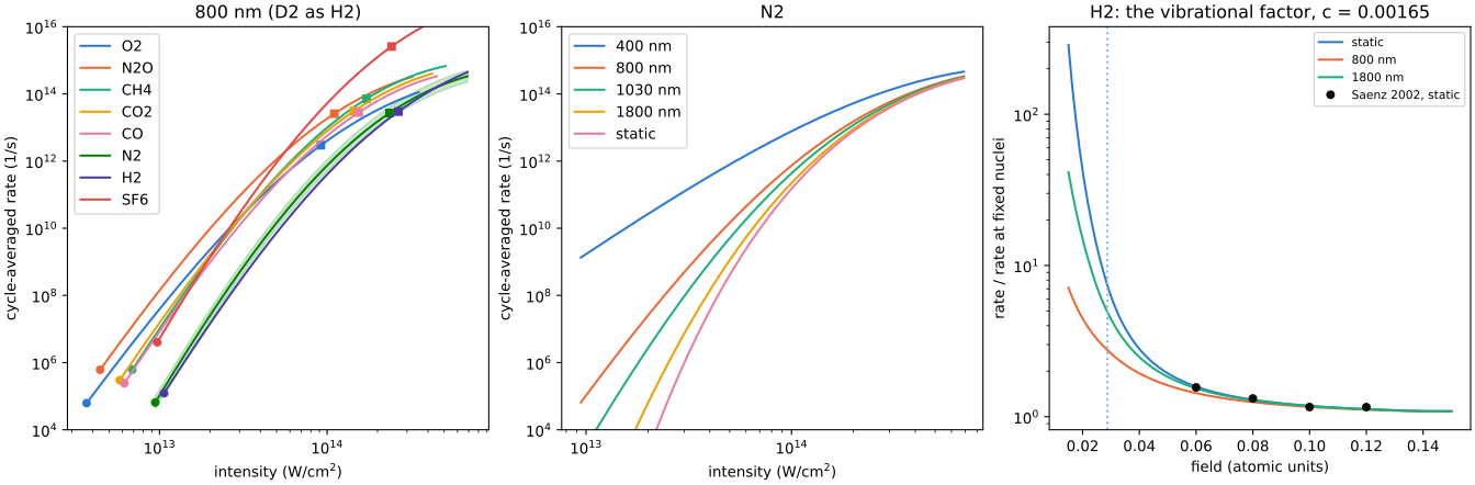
Left: the cycle-averaged rate of each molecule at 800 nm against the intensity, up to 1.5 times the barrier-suppression field, the range over which N2’s correction at finite field holds its all-electron rates within 13 % (with N2’s alpha the rate stops rising at 1.7 times; TC-683). The circles mark a Keldysh parameter of 1 and the squares the barrier-suppression intensity. The band around N2 is its uncertainty factor, 1.5 (CO’s too); O2’s and CH4’s, fitted to coupled-cluster rates, is 2 (TC-698); CO2’s and N2O’s is 3, as their correction is N2’s untested (TC-680). SF6, above the others by one to two orders of magnitude for its ionisation energy, is a prediction of its structure coefficients that nothing tests (factor 10; TC-684).

Centre: N2 at 400, 800, 1030 and 1800 nm and in a static field (the cycle average of the static rate). The rate tends to the static one as the intensity rises and the Keldysh parameter falls. This dependence on the frequency is that of the noble gases, which one-electron and helium calculations test; no calculation of a molecule does (TC-680).

Right: H2’s vibrational factor \(V\), the rate over the rate at fixed nuclei, against the field: static (with Saenz’s (2002) rates averaged over the vibrational ground state, over his rates at 1.4 bohr) and at 800 and 1800 nm. At finite frequency the rate depends less on the ionisation energy, and so on the bond length, than in a static field, and \(V\) is smaller. Left of the dotted line the static factor is continued as the contribution of one bond length, two standard deviations out in the ground state, so that the rate still falls to zero with the field (TC-679).

import math
import warnings
from dataclasses import replace

import matplotlib.pyplot as plt
import numpy as np
from _helpers import COLOURS
from matplotlib.ticker import NullFormatter

from optmat.constants import AU_FIELD, EPS0, C
from optmat.exceptions import ModelRangeWarning
from optmat.gas.molecular_ionisation_rates import molecular_rate_model
from optmat.gas.molecular_ionisation_validation import vibrational_factors

MOLECULES = ("O2", "N2O", "CH4", "CO2", "CO", "N2", "H2", "SF6")


def intensity_of(field):
    """Return the intensity in W/cm^2 of a field's amplitude in V/m."""
    return 0.5 * EPS0 * C * field**2 / 1e4


fig, axes = plt.subplots(1, 3, figsize=(14, 4.6), layout="constrained")
for colour, gas in zip(COLOURS, MOLECULES, strict=False):
    model = molecular_rate_model(gas, 800e-9)
    field = np.geomspace(
        0.2 * model.barrier_suppression_field, model.maximum_field, 200
    )
    rate = model.cycle_averaged_rate(field)
    axes[0].loglog(intensity_of(field), rate, color=colour, label=gas)
    if gas == "N2":
        factor = model.uncertainty_factor
        axes[0].fill_between(
            intensity_of(field), rate / factor, rate * factor, color=colour, alpha=0.2
        )
    unity = np.interp(-1.0, -model.keldysh(field)[::-1], field[::-1])
    for mark, at in (("o", unity), ("s", model.barrier_suppression_field)):
        axes[0].loglog(
            intensity_of(at), model.cycle_averaged_rate(at), mark, color=colour, ms=5
        )
axes[0].set_ylim(1e4, 1e16)
axes[0].set_xlabel("intensity (W/cm$^2$)")
axes[0].set_ylabel("cycle-averaged rate (1/s)")
axes[0].set_title("800 nm (D2 as H2)")
axes[0].xaxis.set_minor_formatter(NullFormatter())
axes[0].legend()

nitrogen = molecular_rate_model("N2", 800e-9)
field = np.geomspace(
    0.2 * nitrogen.barrier_suppression_field, nitrogen.maximum_field, 200
)
for colour, wavelength in zip(
    COLOURS, (400e-9, 800e-9, 1030e-9, 1800e-9, math.inf), strict=False
):
    label = "static" if math.isinf(wavelength) else f"{wavelength * 1e9:.0f} nm"
    rate = nitrogen.at_wavelength(wavelength).cycle_averaged_rate(field)
    axes[1].loglog(intensity_of(field), rate, color=colour, label=label)
axes[1].set_ylim(1e4, 1e16)
axes[1].set_xlabel("intensity (W/cm$^2$)")
axes[1].set_ylabel("cycle-averaged rate (1/s)")
axes[1].set_title("N2")
axes[1].xaxis.set_minor_formatter(NullFormatter())
axes[1].legend()

hydrogen = molecular_rate_model("H2", math.inf)
field_au = np.linspace(0.015, 0.15, 200)
with warnings.catch_warnings():
    # H2's correction was fitted to 0.12 au, 1.3 times its barrier-suppression field.
    warnings.simplefilter("ignore", ModelRangeWarning)
    for colour, wavelength in zip(COLOURS, (math.inf, 800e-9, 1800e-9), strict=False):
        model = hydrogen.at_wavelength(wavelength)
        fixed = replace(model, vibrational_constant=0.0)
        field = field_au * AU_FIELD
        factor = model.instantaneous_rate(field) / fixed.instantaneous_rate(field)
        label = "static" if math.isinf(wavelength) else f"{wavelength * 1e9:.0f} nm"
        axes[2].semilogy(field_au, factor, color=colour, label=label)
saenz = vibrational_factors()
axes[2].semilogy(
    saenz.field / AU_FIELD,
    saenz.expected,
    "o",
    color="#0b0b0b",
    ms=5,
    label="Saenz 2002, static",
)
tail = math.sqrt(2 * hydrogen.vibrational_constant) / 2
axes[2].axvline(tail, color="#86b6ef", ls=":")
axes[2].set_xlabel("field (atomic units)")
axes[2].set_ylabel("rate / rate at fixed nuclei")
axes[2].set_title(f"H2: the vibrational factor, c = {hydrogen.vibrational_constant:g}")
axes[2].legend(fontsize=8)
plt.show()