Ionisation: the rates of the noble gases

The default ionisation rates (optmat.gas.ionisation_rates.ionisation_rate_model()).

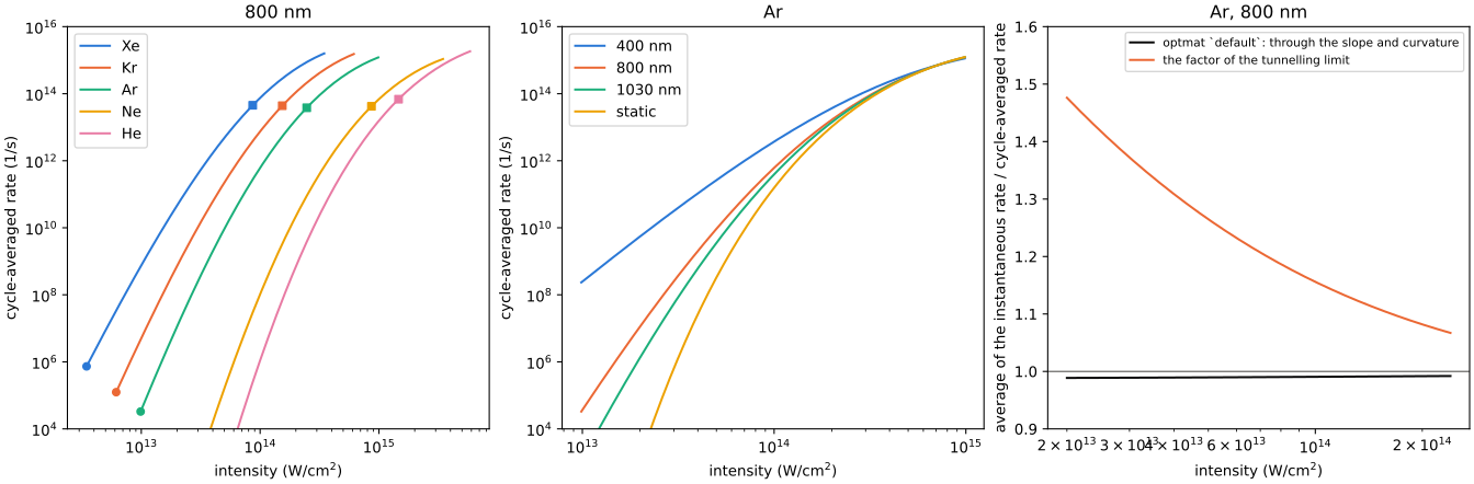
Left: the cycle-averaged rate of each gas at 800 nm against the intensity, up to twice the barrier-suppression field, the range over which the static correction was fitted. The circles mark a Keldysh parameter of 1 and the squares the barrier-suppression intensity.

Centre: argon at 400, 800 and 1030 nm and in a static field (the cycle average of the static rate). The rate tends to the static one as the intensity rises and the Keldysh parameter falls.

Right: the average of the instantaneous rate over a cycle, over the cycle-averaged rate, for argon at 800 nm. In the default model the two are related through the local slope and curvature of the rate (optmat.gas.ionisation_rates.cycle_average()) and agree to 3 %. With the factor of the tunnelling limit, \((3F/\pi F_0)^{1/2}\), which the literature’s forms use (here ppt_larochelle), the instantaneous rate ionises more over a cycle than the cycle-averaged rate it was made from (TC-662).

import math

import matplotlib.pyplot as plt
import numpy as np
from _helpers import COLOURS

from optmat.constants import EPS0, C
from optmat.gas.ionisation_rates import ionisation_rate_model
from optmat.gas.ionisation_validation import amplitude


def intensity_of(field):
    """Return the intensity in W/cm^2 of a field's amplitude in V/m."""
    return 0.5 * EPS0 * C * field**2 / 1e4


fig, axes = plt.subplots(1, 3, figsize=(14, 4.6), layout="constrained")
for colour, gas in zip(COLOURS, ("Xe", "Kr", "Ar", "Ne", "He"), strict=False):
    model = ionisation_rate_model(gas, 800e-9)
    field = np.geomspace(
        0.2 * model.barrier_suppression_field, model.maximum_field, 200
    )
    rate = model.cycle_averaged_rate(field)
    axes[0].loglog(intensity_of(field), rate, color=colour, label=gas)
    unity = np.interp(-1.0, -model.keldysh(field)[::-1], field[::-1])
    for mark, at in (("o", unity), ("s", model.barrier_suppression_field)):
        axes[0].loglog(
            intensity_of(at), model.cycle_averaged_rate(at), mark, color=colour, ms=5
        )
axes[0].set_ylim(1e4, 1e16)
axes[0].set_xlabel("intensity (W/cm$^2$)")
axes[0].set_ylabel("cycle-averaged rate (1/s)")
axes[0].set_title("800 nm")
axes[0].legend()

argon = ionisation_rate_model("Ar", 800e-9)
field = np.geomspace(0.2 * argon.barrier_suppression_field, argon.maximum_field, 200)
for colour, wavelength in zip(
    COLOURS, (400e-9, 800e-9, 1030e-9, math.inf), strict=False
):
    label = "static" if math.isinf(wavelength) else f"{wavelength * 1e9:.0f} nm"
    rate = argon.at_wavelength(wavelength).cycle_averaged_rate(field)
    axes[1].loglog(intensity_of(field), rate, color=colour, label=label)
axes[1].set_ylim(1e4, 1e16)
axes[1].set_xlabel("intensity (W/cm$^2$)")
axes[1].set_ylabel("cycle-averaged rate (1/s)")
axes[1].set_title("Ar")
axes[1].legend()

phase = np.linspace(0, math.pi / 2, 2001)
intensity = np.geomspace(2e17, 2.4e18, 30)
for name, colour, label in (
    ("default", "#0b0b0b", "optmat `default`: through the slope and curvature"),
    ("ppt_larochelle", COLOURS[1], "the factor of the tunnelling limit"),
):
    model = ionisation_rate_model("Ar", 800e-9, name)
    ratio = [
        np.trapezoid(model.instantaneous_rate(peak * np.cos(phase)), phase)
        * 2
        / math.pi
        / float(model.cycle_averaged_rate(peak))
        for peak in amplitude(intensity)
    ]
    axes[2].semilogx(intensity / 1e4, ratio, color=colour, label=label)
axes[2].axhline(1.0, color="#52514e", lw=0.8)
axes[2].set_ylim(0.9, 1.6)
axes[2].set_xlabel("intensity (W/cm$^2$)")
axes[2].set_ylabel("average of the instantaneous rate / cycle-averaged rate")
axes[2].set_title("Ar, 800 nm")
axes[2].legend(fontsize=8)
plt.show()