Two-photon ionisation of the noble gases

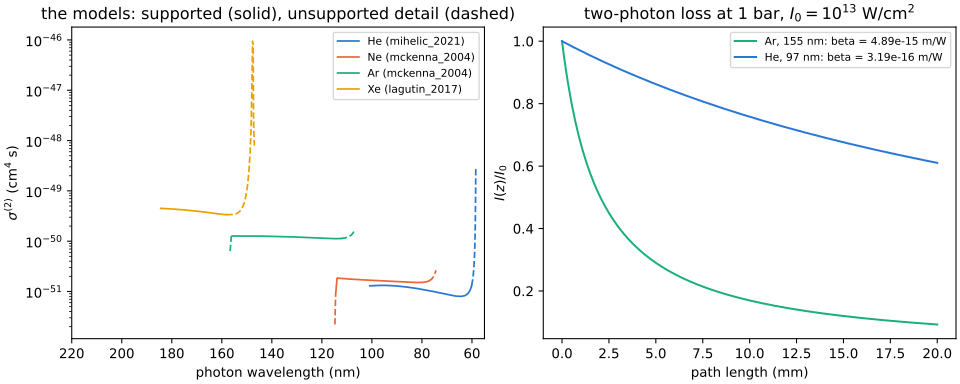
The two-photon ionisation cross sections of the models of optmat.gas.two_photon.two_photon_ionisation_model() (OEP 6, Phase 1), each the curated reference curve the author approved (TC-943):

• helium: Mihelič and Horvat;

• neon and argon: McKenna and van der Hart;

• xenon: Lagutin et al.

Krypton has none (OEP 6, Q2).

Left: \(\sigma^{(2)}\) against the vacuum wavelength of one photon, from the two-photon threshold \(2hc/I_p\) to the first one-photon resonance. Solid lines are supported values; dashed lines are unsupported detail, the resonance wing and, for an LS-coupled reference, the band between the ion’s two thresholds. Gaps are unavailable, such as xenon between its two thresholds.

Right: the intensity of a flat-top plane wave after a path \(z\) in the gas at 1 bar and 293.15 K, \(I(z) = I_0 / (1 + \beta I_0 z)\) with \(\beta = 2 N \sigma^{(2)} / \hbar\omega\), for \(I_0 = 10^{13}\) W/cm² in argon at 155 nm and helium at 97 nm. This is the two-photon loss of a prescribed field, not a prediction of resonant-dispersive-wave generation: a propagation model decides how the field evolves. The time dependence of the loss within a broadband pulse is a documented gap (TC-903).

import warnings

import matplotlib.pyplot as plt
import numpy as np
from _helpers import COLOURS

from optmat.constants import BAR, K_B, C
from optmat.exceptions import ModelRangeWarning
from optmat.gas.two_photon import two_photon_ionisation_model

DENSITY = BAR / (K_B * 293.15)  # m^-3
fig, (left, right) = plt.subplots(1, 2, figsize=(10, 4), constrained_layout=True)
for colour, gas in zip(COLOURS, ("He", "Ne", "Ar", "Xe"), strict=False):
    model = two_photon_ionisation_model(gas)
    nm = np.linspace(2 * np.pi * C / model.thresholds[0].omega * 1e9 + 0.5, 50, 4000)
    omega = 2 * np.pi * C / (nm * 1e-9)
    with warnings.catch_warnings():
        warnings.simplefilter("ignore", ModelRangeWarning)
        sigma = model.cross_section(omega) * 1e8  # cm^4 s
    labels = model.region(omega)
    for label, style in (("supported", "-"), ("unsupported_detail", "--")):
        shown = np.where(labels == label, sigma, np.nan)
        left.semilogy(
            nm,
            shown,
            style,
            color=colour,
            lw=1.3,
            label=f"{gas} ({model.reference.datasets[0].split('/')[0]})"
            if label == "supported"
            else None,
        )
left.set_xlim(220, 55)
left.set_xlabel("photon wavelength (nm)")
left.set_ylabel(r"$\sigma^{(2)}$ (cm$^4$ s)")
left.set_title("the models: supported (solid), unsupported detail (dashed)")
left.legend(fontsize=8)

z = np.linspace(0, 0.02, 200)  # m
intensity = 1e17  # W/m^2, 1e13 W/cm^2
for colour, gas, nm in ((COLOURS[2], "Ar", 155.0), (COLOURS[0], "He", 97.0)):
    model = two_photon_ionisation_model(gas)
    omega = 2 * np.pi * C / (nm * 1e-9)
    beta = float(model.loss_coefficient(omega, DENSITY))
    right.plot(
        z * 1e3,
        1 / (1 + beta * intensity * z),
        color=colour,
        label=f"{gas}, {nm:g} nm: beta = {beta:.2e} m/W",
    )
right.set_xlabel("path length (mm)")
right.set_ylabel(r"$I(z) / I_0$")
right.set_title(r"two-photon loss at 1 bar, $I_0 = 10^{13}$ W/cm$^2$")
right.legend(fontsize=8)
plt.show()