Ionisation: the measured yields of argon, krypton and xenon

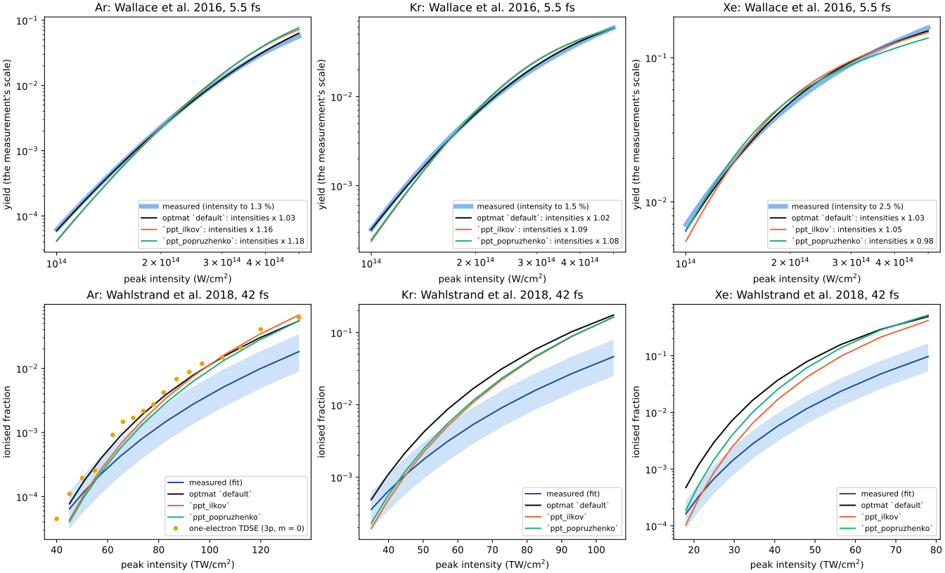
Two measurements have an intensity scale that does not rest on a rate model.

Top: Wallace et al. (2016), 800 nm, 5.5 fs, a thin atomic beam across the focus. The intensity is fixed by the yield of atomic hydrogen to 1.3 % (Ar), 1.5 % (Kr) and 2.5 % (Xe); the scale of the yield is free. The grey line is the measurement (the authors’ fit, their eq. 4). The models’ yields are averaged over the focus and over the carrier-envelope phase, and scaled in amplitude to the measurement; what is tested is where the yield bends towards saturation. The legend gives the factor by which the intensities must be multiplied for the model to match (optmat.gas.ionisation_validation.intensity_scale_test()); the default matches at intensity factors 1.033, 1.023 and 1.026 for Ar, Kr and Xe respectively. All three differ from unity by more than the stated calibration. The Kr and Xe electron counts were selected using these yields (TC-848, TC-850).

Bottom: Wahlstrand et al. (2018), 800 nm, 42 fs, the absolute yield from the refractive index of the plasma, at a local intensity known to 13 %. The grey line is the measurement (the fit of the Supplemental Material) and the band its intensity’s uncertainty. The default model lies above it by 1.2 to 3.1 (Ar), 1.4 to 3.8 (Kr) and 2.9 to 6.8 (Xe). For argon the circles are a time-dependent calculation of one electron (3p, m = 0) in the same pulse, its ionised fraction: already 1.3 to 4.1 times the measured yield of the atom (TC-702).

The two measurements disagree with each other by about 3 in the rate, which is open (TC-660).

import warnings

import matplotlib.pyplot as plt
import numpy as np
from _helpers import COLOURS

from optmat.exceptions import ModelRangeWarning
from optmat.gas.ionisation_validation import (
    intensity_scale_test,
    long_pulse_yield,
    measured_yields,
)

MODELS = {
    "default": ("optmat `default`", "#0b0b0b"),
    "ppt_ilkov": ("`ppt_ilkov`", COLOURS[1]),
    "ppt_popruzhenko": ("`ppt_popruzhenko`", COLOURS[2]),
}
INTENSITY_UNCERTAINTY = 0.13  # Wahlstrand et al. 2018, caption of Fig. 3

fig, axes = plt.subplots(2, 3, figsize=(14, 8.5), layout="constrained")
with warnings.catch_warnings():
    # The yields run into saturation, beyond the range of the static correction.
    warnings.simplefilter("ignore", ModelRangeWarning)
    for column, gas in enumerate(("Ar", "Kr", "Xe")):
        top, bottom = axes[:, column]
        for name, (label, colour) in MODELS.items():
            test = intensity_scale_test(gas, name)
            if name == "default":
                top.loglog(
                    test.intensity / 1e4,
                    test.measured,
                    color="#86b6ef",
                    lw=5,
                    label=f"measured (intensity to {100 * test.calibration:.1f} %)",
                )
            # The model at the measurement's own intensities, with the amplitude
            # that fits it best.
            top.loglog(
                test.intensity / 1e4,
                test.unscaled,
                color=colour,
                label=f"{label}: intensities x {test.scale:.2f}",
            )
        top.set_xlabel("peak intensity (W/cm$^2$)")
        top.set_ylabel("yield (the measurement's scale)")
        top.set_title(f"{gas}: Wallace et al. 2016, 5.5 fs")
        top.legend(fontsize=8, loc="lower right")

        measured = measured_yields(gas)
        x = measured.x / 1e16
        power = np.log(measured.expected[-1] / measured.expected[0]) / np.log(
            x[-1] / x[0]
        )
        bottom.fill_between(
            x,
            measured.expected * (1 - INTENSITY_UNCERTAINTY) ** power,
            measured.expected * (1 + INTENSITY_UNCERTAINTY) ** power,
            color="#86b6ef",
            alpha=0.4,
            lw=0,
        )
        bottom.semilogy(x, measured.expected, color="#184f95", label="measured (fit)")
        for name, (label, colour) in MODELS.items():
            comparison = measured_yields(gas, name, intensities=list(measured.x))
            bottom.semilogy(x, comparison.predicted, color=colour, label=label)
        if gas == "Ar":
            # One electron, the 3p m = 0 orbital, in the same pulse (TC-702).
            tdse = long_pulse_yield()
            bottom.semilogy(
                tdse.x / 1e16,
                tdse.expected,
                "o",
                color=COLOURS[3],
                ms=4,
                label="one-electron TDSE (3p, m = 0)",
            )
        bottom.set_xlabel("peak intensity (TW/cm$^2$)")
        bottom.set_ylabel("ionised fraction")
        bottom.set_title(f"{gas}: Wahlstrand et al. 2018, 42 fs")
        bottom.legend(fontsize=8, loc="lower right")
plt.show()