Ozone: the fitted model

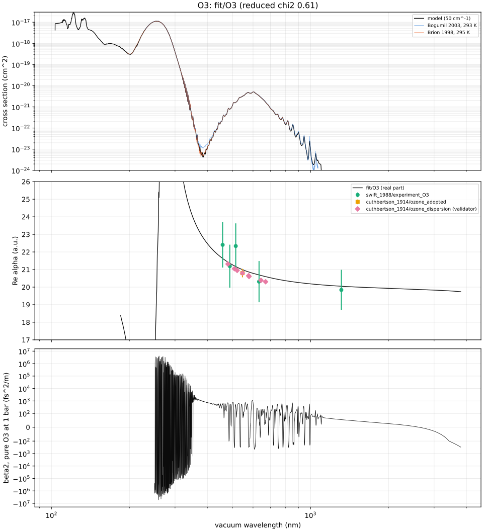
The O3 model (fit/O3) absorbs. Its imaginary part is the measured absorption spectrum (Serdyuchenko et al. 2014 at 293 K from 213 nm, Yoshino et al. 1993, Mason et al. 1996 and Ogawa & Cook 1958 to 12 eV), smoothed with a 50 cm^-1 Gaussian. Its real part is that spectrum’s Kramers-Kronig transform, plus:

• Kumar & Thakkar’s interval strengths above 20.6 eV;

• one oscillator for 12-20.6 eV, fitted to Swift et al., the Cuthbertsons’ level and the ab initio static value plus Naves et al.’s zero-point vibrational correction;

• HITRAN’s vibrational bands.

Top: the cross section of the model, with Bogumil’s and Brion’s independent spectra.

Middle: the real polarizability against the refractivity data (the Cuthbertsons’ dispersion is a validator).

Bottom: the group-velocity dispersion of pure ozone at 1 bar and 20 C. It is set by the band structure of the measured spectrum and is uncertain by tens of per cent at 343 and 800 nm (see Accuracy); clear of the bands it is known to 1 %.

Text(0.5, 1.0, 'O3: fit/O3 (reduced chi2 0.61)')

import gzip

import matplotlib.pyplot as plt
import numpy as np
from _helpers import COLOURS, LINE_COLOURS, MARKERS

from optmat.conditions import State
from optmat.constants import AU_ANGULAR_FREQUENCY, AU_POLARIZABILITY, EPS0, C
from optmat.datasets import DATA_DIRECTORY, datasets
from optmat.gas import reduction
from optmat.gas.eos import number_density
from optmat.gas.models.fitted import fitted_models
from optmat.gas.models.oscillator import angular_frequency_au

model = fitted_models()["fit/O3"]
absorption = model.absorption
assert absorption is not None

fig, (top, middle, bottom) = plt.subplots(
    3, 1, sharex=True, figsize=(10, 11), layout="constrained", height_ratios=(2, 2, 2)
)

# Cross sections: the model's (smoothed) and two independent spectra.
inside = absorption.wavenumber_cm > 1e7 / 1100.0
top.semilogy(
    1e7 / absorption.wavenumber_cm[inside],
    absorption.sigma_m2[inside] * 1e4,
    color=LINE_COLOURS[0],
    linewidth=1.0,
    label="model (50 cm^-1)",
)
external = DATA_DIRECTORY / "external" / "mainz_uvvis"
for colour, (label, name) in zip(
    COLOURS[:2],
    [
        ("Bogumil 2003, 293 K", "O3_Bogumil2003_293K_230-1070nm.txt.gz"),
        ("Brion 1998, 295 K", "O3_Brion1998_295K_195.00-830.00nm.txt.gz"),
    ],
    strict=True,
):
    with gzip.open(external / name, "rt", encoding="utf-8") as handle:
        table = np.loadtxt(handle)
    top.semilogy(
        table[:, 0], table[:, 1], color=colour, linewidth=0.5, alpha=0.7, label=label
    )
top.set_ylim(1e-24, 3e-17)
top.set_ylabel("cross section (cm^2)")
top.legend(fontsize=7)

# Real polarizability against the refractivity data.
grid = np.geomspace(185e-9, 3.8e-6, 3000)
alpha = model.complex_polarizability(grid, warn=False) / AU_POLARIZABILITY
middle.plot(
    grid * 1e9,
    np.real(alpha),
    color=LINE_COLOURS[0],
    linewidth=1.0,
    label="fit/O3 (real part)",
)
shown = [
    "swift_1988/experiment_O3",
    "cuthbertson_1914/ozone_adopted",
    "cuthbertson_1914/ozone_dispersion",
]
by_key = {d.key: d for d in datasets("O3")}
for index, key in enumerate(shown):
    dataset = by_key[key]
    values = reduction.polarizability(dataset) / AU_POLARIZABILITY
    sigma = reduction.polarizability_uncertainty(dataset) / AU_POLARIZABILITY
    middle.errorbar(
        dataset.vacuum_wavelength() * 1e9,
        values,
        yerr=np.where(np.isfinite(sigma), sigma, 0.0),
        fmt=MARKERS[index],
        color=COLOURS[index + 2],
        markersize=5,
        label=key + (" (validator)" if "dispersion" in key else ""),
    )
middle.set_ylim(17, 26)
middle.set_ylabel("Re alpha (a.u.)")
middle.legend(fontsize=7)

# Group-velocity dispersion of pure ozone at 1 bar, 293 K (dilute limit).
state = State(1e5, 293.15)
density = number_density("O3", state, ideal=True)
omega = angular_frequency_au(grid)
second = model.dispersion_au(omega, 2)
beta2 = (
    density * AU_POLARIZABILITY * second / (2 * EPS0 * C * AU_ANGULAR_FREQUENCY) * 1e30
)
shown_range = grid > 250e-9  # inside the Hartley band the absorption dominates
bottom.plot(
    grid[shown_range] * 1e9, beta2[shown_range], color=LINE_COLOURS[0], linewidth=0.6
)
bottom.set_yscale("symlog", linthresh=100.0)
bottom.set_ylabel("beta2, pure O3 at 1 bar (fs^2/m)")
bottom.set_xscale("log")
bottom.set_xlabel("vacuum wavelength (nm)")
for axis in (top, middle, bottom):
    axis.grid(which="both", alpha=0.25)
top.set_title(f"O3: fit/O3 (reduced chi2 {model.reduced_chi2:.2f})")