Linear density scaling against Lorentz-Lorenz

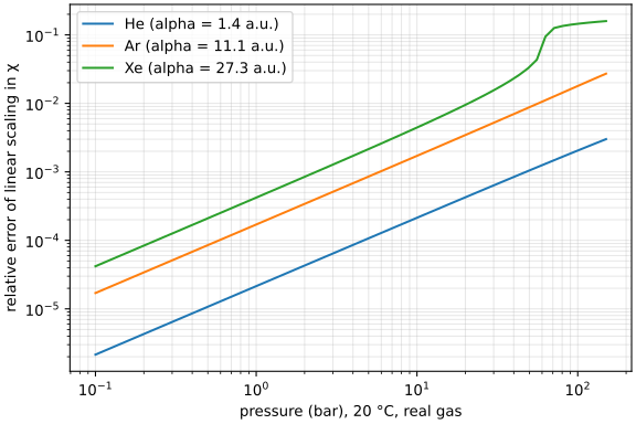
The refractive index of a gas at number density \(N\) follows from the per-particle polarizability \(\alpha\) through the Lorentz-Lorenz relation. The linear scaling \(\chi = N\alpha/\varepsilon_0\) is its dilute limit. This figure shows the relative error of linear scaling in \(\chi = n^2 - 1\) against pressure, for a polarizability typical of each gas.

The polarizabilities are illustrative round numbers (atomic units), not curated data: the error depends only on \(\chi\) itself, \(1/(1-y) - 1\) with \(y = N\alpha/(3\varepsilon_0)\).

import matplotlib.pyplot as plt
import numpy as np

from optmat.conditions import State
from optmat.constants import AU_POLARIZABILITY, BAR
from optmat.gas.eos import number_density
from optmat.gas.lorentz_lorenz import susceptibility, susceptibility_dilute

pressures = np.geomspace(0.1, 150.0, 60)  # bar
fig, ax = plt.subplots(figsize=(6, 4), layout="constrained")
for gas, alpha_au in [("He", 1.4), ("Ar", 11.1), ("Xe", 27.3)]:
    errors = []
    for p in pressures:
        density = number_density(gas, State(p * BAR, 293.15))
        alpha = alpha_au * AU_POLARIZABILITY
        exact = susceptibility(alpha, density)
        errors.append(1 - susceptibility_dilute(alpha, density) / exact)
    ax.loglog(pressures, errors, label=f"{gas} (alpha = {alpha_au} a.u.)")
ax.set_xlabel("pressure (bar), 20 °C, real gas")
ax.set_ylabel("relative error of linear scaling in χ")
ax.legend()
ax.grid(which="both", alpha=0.3)
plt.show()