Ionisation: the Coulomb factor against Schrödinger calculations

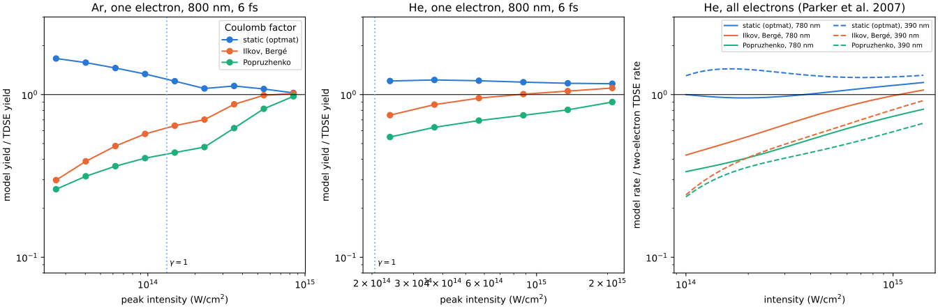
The rate of Perelomov, Popov and Terent’ev is that of a short-range potential times a Coulomb factor. This figure compares three analytic forms (optmat.gas.ionisation_rates.coulomb_factor()). Here each is compared with time-dependent Schrödinger calculations, with everything else the same: one electron in the \(m = 0\) orbital, Tong, Zhao and Lin’s coefficient and Tong and Lin’s static correction, so that all three have the same static limit.

Left and centre: the yield of a 6 fs pulse at 800 nm, over the ionised fraction of calculations for one electron in Tong and Lin’s potentials (travers_2026_trecx): the population that has left the bound states up to n = 10 at the end of the pulse.

Right: the cycle-averaged rate of helium at 780 nm (solid) and 390 nm (dashed), over Parker et al.’s (2007) fits of their two-electron calculations, with the default’s effective number of electrons.

None of these three forms follows all the calculations. The static factor, \((2F_0/F)^{2n^*}\), is 1.1 to 1.7 times above them for argon at Keldysh parameters 0.6 to 2.3, the most at the largest, and 1.2 times above for helium. The factor \((1 + \gamma^2)^{-n^*}\) of Ilkov et al. and Bergé et al., and Popruzhenko et al.’s \((1 + 2\gamma/e)^{-2n^*}\), cross them near \(\gamma = 1\): below them by 2 to 3 at \(\gamma \approx 2\), above by up to 1.7 at \(\gamma \approx 0.6\) (TC-653, TC-812).

The empirical frequency-dependent factor adopted in TC-848 is assessed separately in Noble-gas ionisation: one-electron calculations; it is not one of the three curves here.

import dataclasses
import warnings

import matplotlib.pyplot as plt
import numpy as np
from _helpers import COLOURS

from optmat.constants import AU_ANGULAR_FREQUENCY
from optmat.exceptions import ModelRangeWarning
from optmat.gas.ionisation_rates import ionisation_rate_model
from optmat.gas.ionisation_validation import (
    amplitude,
    parker_rate_au,
    pulse_yield,
    tdse_yields,
)

FORMS = {
    "static": ("static (optmat)", COLOURS[0]),
    "ilkov": ("Ilkov, Bergé", COLOURS[1]),
    "popruzhenko": ("Popruzhenko", COLOURS[2]),
}

fig, axes = plt.subplots(1, 3, figsize=(14, 4.6), layout="constrained")
with warnings.catch_warnings():
    # The yields run into saturation, beyond the range of the static correction.
    warnings.simplefilter("ignore", ModelRangeWarning)
    for axis, gas in zip(axes[:2], ("Ar", "He"), strict=True):
        ionised = tdse_yields(gas)[0]  # 800 nm, 6 fs
        base = ionisation_rate_model(gas, ionised.wavelength, "one_electron")
        for form, (label, colour) in FORMS.items():
            model = dataclasses.replace(base, coulomb=form)
            predicted = np.array(
                [pulse_yield(model, peak, 6e-15, carrier=True) for peak in ionised.x]
            )
            axis.semilogx(
                ionised.x / 1e4,
                predicted / ionised.expected,
                color=colour,
                marker="o",
                label=label,
            )
        axis.axhline(1.0, color="#0b0b0b", lw=0.8)
        axis.set_yscale("log")
        axis.set_ylim(0.08, 3)
        axis.set_xlabel("peak intensity (W/cm$^2$)")
        axis.set_ylabel("model yield / TDSE yield")
        axis.set_title(f"{gas}, one electron, 800 nm, 6 fs")
        unity = np.interp(
            -1.0,
            -base.keldysh(amplitude(np.geomspace(1e17, 1e20, 300))),
            np.geomspace(1e13, 1e16, 300),
        )
        axis.axvline(unity, color="#86b6ef", ls=":")
        axis.annotate(
            r"$\gamma = 1$",
            (unity, 0.09),
            xytext=(3, 0),
            textcoords="offset points",
            fontsize=8,
        )
    axes[0].legend(title="Coulomb factor", fontsize=8)

    intensity = np.geomspace(1e18, 1.4e19, 40)
    for wavelength, style in ((780, "-"), (390, "--")):
        base = ionisation_rate_model("He", wavelength * 1e-9)
        expected = parker_rate_au(intensity, wavelength)
        for form, (label, colour) in FORMS.items():
            model = dataclasses.replace(base, coulomb=form)
            rate = (
                model.cycle_averaged_rate(amplitude(intensity)) / AU_ANGULAR_FREQUENCY
            )
            axes[2].semilogx(
                intensity / 1e4,
                rate / expected,
                color=colour,
                ls=style,
                label=f"{label}, {wavelength} nm",
            )
axes[2].axhline(1.0, color="#0b0b0b", lw=0.8)
axes[2].set_yscale("log")
axes[2].set_ylim(0.08, 3)
axes[2].set_xlabel("intensity (W/cm$^2$)")
axes[2].set_ylabel("model rate / two-electron TDSE rate")
axes[2].set_title("He, all electrons (Parker et al. 2007)")
axes[2].legend(fontsize=7, ncols=2)
plt.show()