Argon: the fitted model

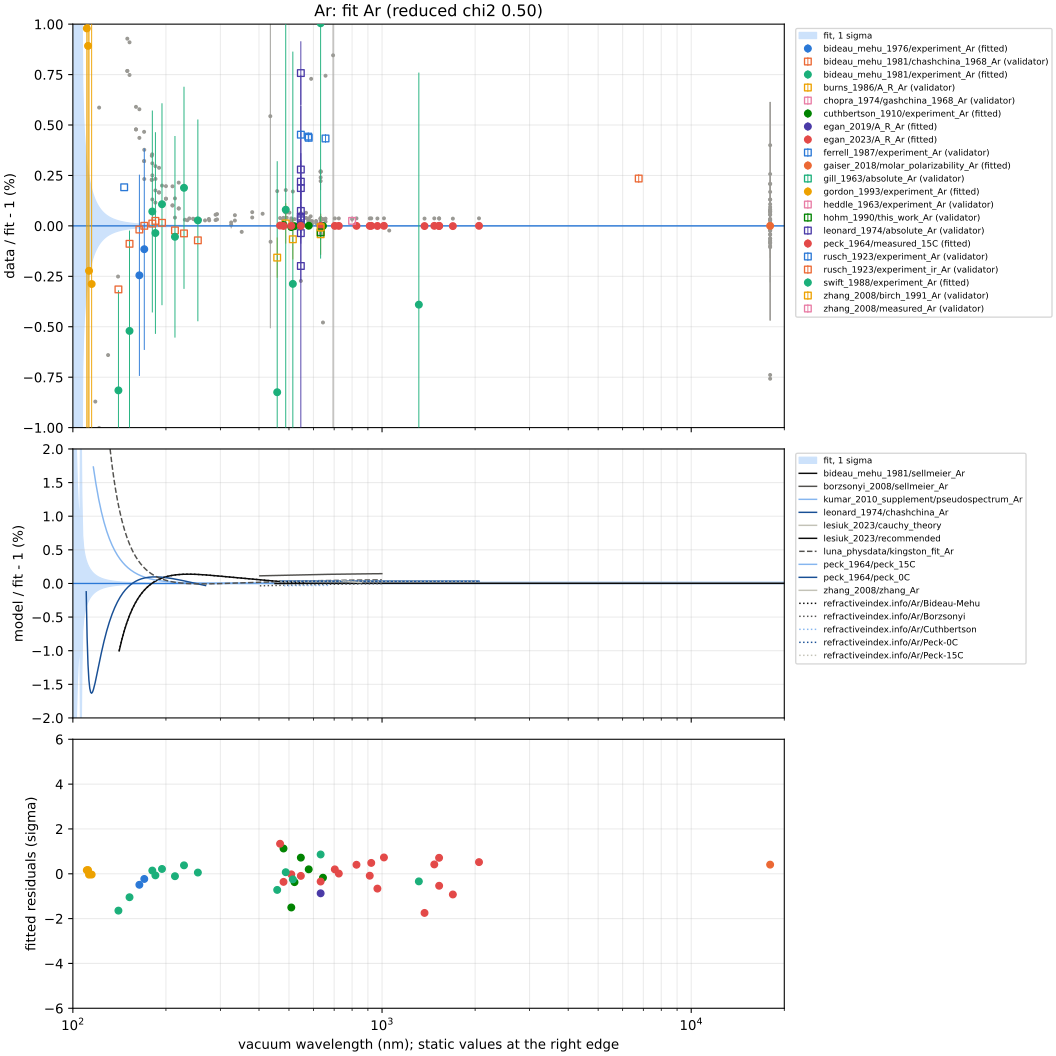
The argon model (fit/Ar): the 104.8 nm and 106.7 nm resonance lines at their NIST energies and two effective oscillators, with the magnetic susceptibility \(\chi_0 = -2.30\times10^{-4}\) a.u. that makes the electric polarizability the refractive one. The absolute level comes from Lesiuk & Jeziorski’s ab initio Cauchy moments, the dielectric static polarizability (Gaiser & Fellmuth, via Lesiuk) and Egan’s refractometry at 633 nm, which agree to a few 1e-5; the shape from 468 nm to 2.06 um from Peck & Fisher, whose level is 3.5e-4 high and is fitted free; the vacuum ultraviolet from Bideau-Mehu and Gordon. Squares are validators, not fitted: Zhang’s comb value at 800 nm (+2.6e-4), Birch at 633 nm, Borzsonyi, Rusch’s infrared point, and the Lyman-alpha values of Gill and Heddle.

Top: direct datasets against the fit, with the fit’s one-sigma band. Configured data use the fitter’s conventions and uncertainties, with fitted scales removed; electric data receive the magnetic term for this comparison. Middle: the published formulas, the recorded luna_physdata fit and refractiveindex.info’s entries against the fit. Bottom: the fitted direct datasets’ normalised residuals; the static dielectric point agrees within one sigma. See Fitting dispersion models for the panel definitions.

from _helpers import fit_overview

fig = fit_overview("Ar", xlim=(100e-9, 20e-6))