Capillary zero-dispersion wavelength

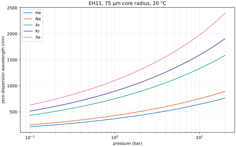
The quantity a change of dispersion model moves most visibly in a gas-filled hollow capillary is the zero-dispersion wavelength (ZDW), where the gas’s normal dispersion balances the waveguide’s anomalous term. For the fundamental EH11 mode of a capillary of core radius \(a\) (Marcatili & Schmeltzer, lossless part)

\[\beta(\omega) = \sqrt{k^2 n_\text{gas}^2(\omega) - u_{01}^2/a^2}, \qquad k = \omega/c,\]

with \(u_{01}\) the first zero of \(J_0\). The ZDW is the root of \(\beta_2 = \mathrm{d}^2\beta/\mathrm{d}\omega^2\). Here \(a = 75\) µm, the gas at 20 °C. The recommended models are evaluated at each pressure with the real-gas density, Lorentz-Lorenz relation and curated refractivity virial. The curves show how pressure shifts the balance between material and waveguide dispersion. See Gas dispersion: accuracy and limitations for uncertainty in the material dispersion. This is the lossless capillary approximation, not a complete waveguide propagation model.

import warnings

import matplotlib.pyplot as plt
import numpy as np
from scipy.optimize import brentq
from scipy.special import jn_zeros

from optmat.conditions import State
from optmat.constants import C
from optmat.exceptions import ModelRangeWarning
from optmat.gas.models.registry import model

RADIUS = 75e-6
U01 = float(jn_zeros(0, 1)[0])
PRESSURES = np.geomspace(0.1e5, 20e5, 25)
TEMPERATURE = 293.15

MODELS = {gas: model(f"fit/{gas}") for gas in ("He", "Ne", "Ar", "Kr", "Xe")}


def beta2(dispersion, omega, state):
    """Return the EH11 mode's beta_2 (s^2/m) by a centred second difference."""
    step = omega * 1e-3
    points = np.array([omega - step, omega, omega + step])
    with warnings.catch_warnings():
        warnings.simplefilter("ignore", ModelRangeWarning)
        n = 1 + dispersion.refractivity(2 * np.pi * C / points, state)
    k = points / C
    beta = np.sqrt((k * n) ** 2 - (U01 / RADIUS) ** 2)
    return (beta[0] - 2 * beta[1] + beta[2]) / step**2


def zdw(dispersion, pressure):
    """Return the zero-dispersion wavelength in nm (NaN if none in 150-3000 nm)."""
    state = State(pressure, TEMPERATURE)
    grid = 2 * np.pi * C / np.geomspace(3000e-9, 150e-9, 200)
    values = np.array([beta2(dispersion, w, state) for w in grid])
    change = np.nonzero(np.diff(np.sign(values)))[0]
    if len(change) == 0:
        return np.nan
    i = change[0]
    root = brentq(lambda w: beta2(dispersion, w, state), grid[i], grid[i + 1])
    return 2 * np.pi * C / root * 1e9


fig, ax = plt.subplots(figsize=(8, 5), layout="constrained")
COLOURS = ["#2a78d6", "#eb6834", "#1baf7a", "#4a3aa7", "#e87ba4"]
for colour, (gas, fitted) in zip(COLOURS, MODELS.items(), strict=True):
    wavelengths = np.array([zdw(fitted, p) for p in PRESSURES])
    ax.plot(PRESSURES / 1e5, wavelengths, color=colour, label=gas)
ax.set_xscale("log")
ax.set_xlabel("pressure (bar)")
ax.set_ylabel("zero-dispersion wavelength (nm)")
ax.legend()
ax.set_title("EH11, 75 µm core radius, 20 °C")
ax.grid(which="both", alpha=0.25)
plt.show()