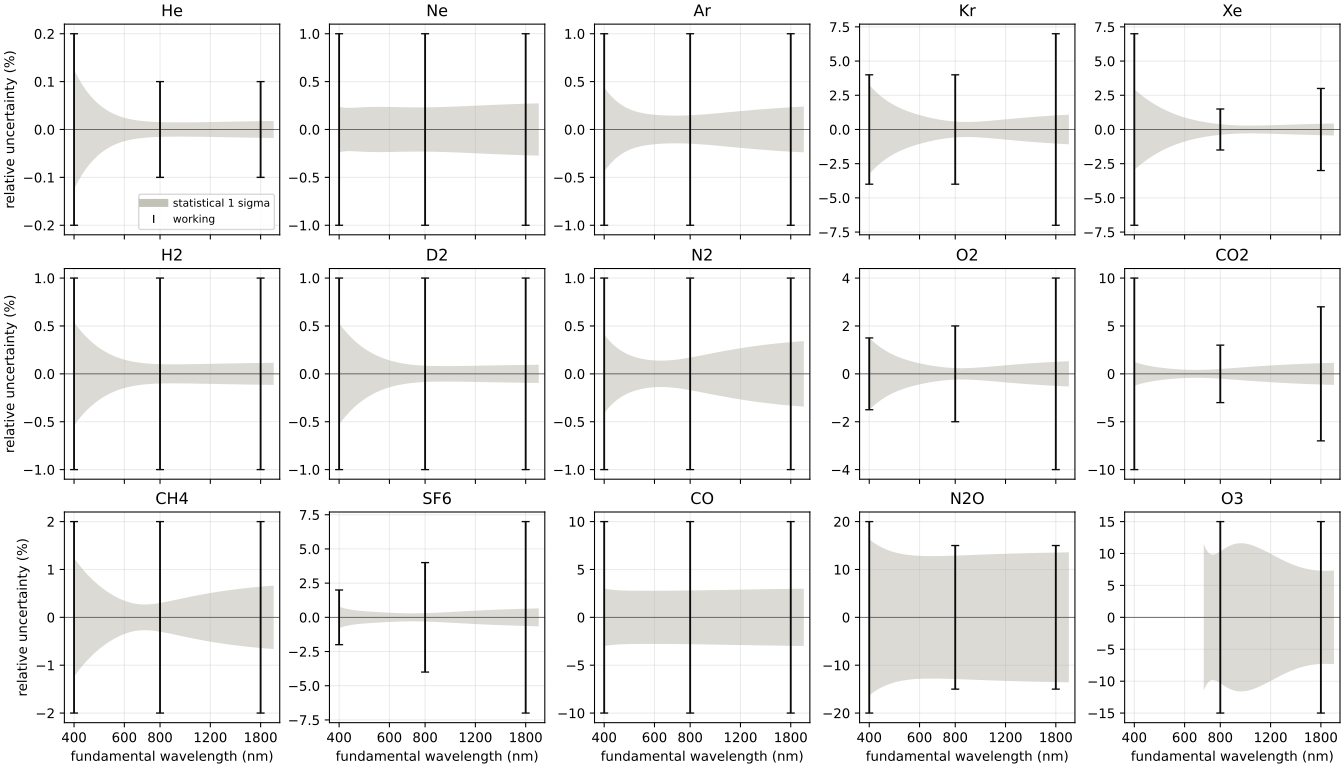
Third-order uncertainty: statistical and working estimates

The shaded band is the fitted Kerr gamma’s propagated statistical one-sigma uncertainty, scaled by the reduced chi-squared where it exceeds one. Bars at 400, 800 and 1800 nm are the working estimates in Third-order accuracy, which include leave-one-out sensitivity and each gas’s systematic floor. They can be much larger than the covariance alone suggests. These are relative uncertainties of the electronic response, not the total nonlinear response or an error bar on extrapolation. Ozone’s model starts at 700 nm.

import warnings

import matplotlib.pyplot as plt
import numpy as np
from _helpers import LINE_COLOURS

from optmat.exceptions import ModelRangeWarning
from optmat.gas.nonlinear import hyperpolarizability_models

# The working estimates of docs/nonlinear_accuracy.md (Kerr at 400, 800 and 1800 nm, %),
# checked against that page by tests/test_nonlinear_accuracy_page.py.
ESTIMATES = {
    "He": (0.2, 0.1, 0.1),
    "Ne": (1, 1, 1),
    "Ar": (1, 1, 1),
    "Kr": (4, 4, 7),
    "Xe": (7, 1.5, 3),
    "H2": (1, 1, 1),
    "D2": (1, 1, 1),
    "N2": (1, 1, 1),
    "O2": (1.5, 2, 4),
    "CO2": (10, 3, 7),
    "CH4": (2, 2, 2),
    "SF6": (2, 4, 7),
    "CO": (10, 10, 10),
    "N2O": (20, 15, 15),
    "O3": (np.nan, 15, 15),
}
models = {gas.value: model for gas, model in hyperpolarizability_models().items()}

fig, axes = plt.subplots(3, 5, figsize=(14, 8), layout="constrained", sharex=True)
for axis, (name, estimates) in zip(axes.flat, ESTIMATES.items(), strict=True):
    model = models[name]
    low = max(400e-9, model.wavelength_range[0])
    wavelength = np.geomspace(low, 2000e-9, 200)
    with warnings.catch_warnings():
        warnings.simplefilter("ignore", ModelRangeWarning)
        kerr = model.gamma_au("kerr", wavelength)
        sigma = model.gamma_sigma_au("kerr", wavelength) / kerr * 100
    nm = wavelength * 1e9
    axis.fill_between(nm, -sigma, sigma, color=LINE_COLOURS[4], alpha=0.6, linewidth=0)
    axis.axhline(0.0, color=LINE_COLOURS[1], linewidth=0.6)
    probe = np.array([400.0, 800.0, 1800.0])
    axis.errorbar(
        probe,
        np.zeros(3),
        yerr=np.array(estimates),
        fmt="none",
        ecolor=LINE_COLOURS[0],
        elinewidth=1.4,
        capsize=3,
    )
    axis.set_title(name)
    axis.set_xscale("log")
    axis.set_xlim(370, 2100)
    axis.set_xticks([400, 600, 800, 1200, 1800], ["400", "600", "800", "1200", "1800"])
    axis.minorticks_off()
    axis.grid(alpha=0.25)
for axis in axes[-1]:
    axis.set_xlabel("fundamental wavelength (nm)")
for axis in axes[:, 0]:
    axis.set_ylabel("relative uncertainty (%)")
axes[0, 0].plot([], [], color=LINE_COLOURS[4], lw=6, label="statistical 1 sigma")
axes[0, 0].plot([], [], color=LINE_COLOURS[0], marker="|", ls="none", label="working")
axes[0, 0].legend(fontsize=8, loc="lower right")
plt.show()