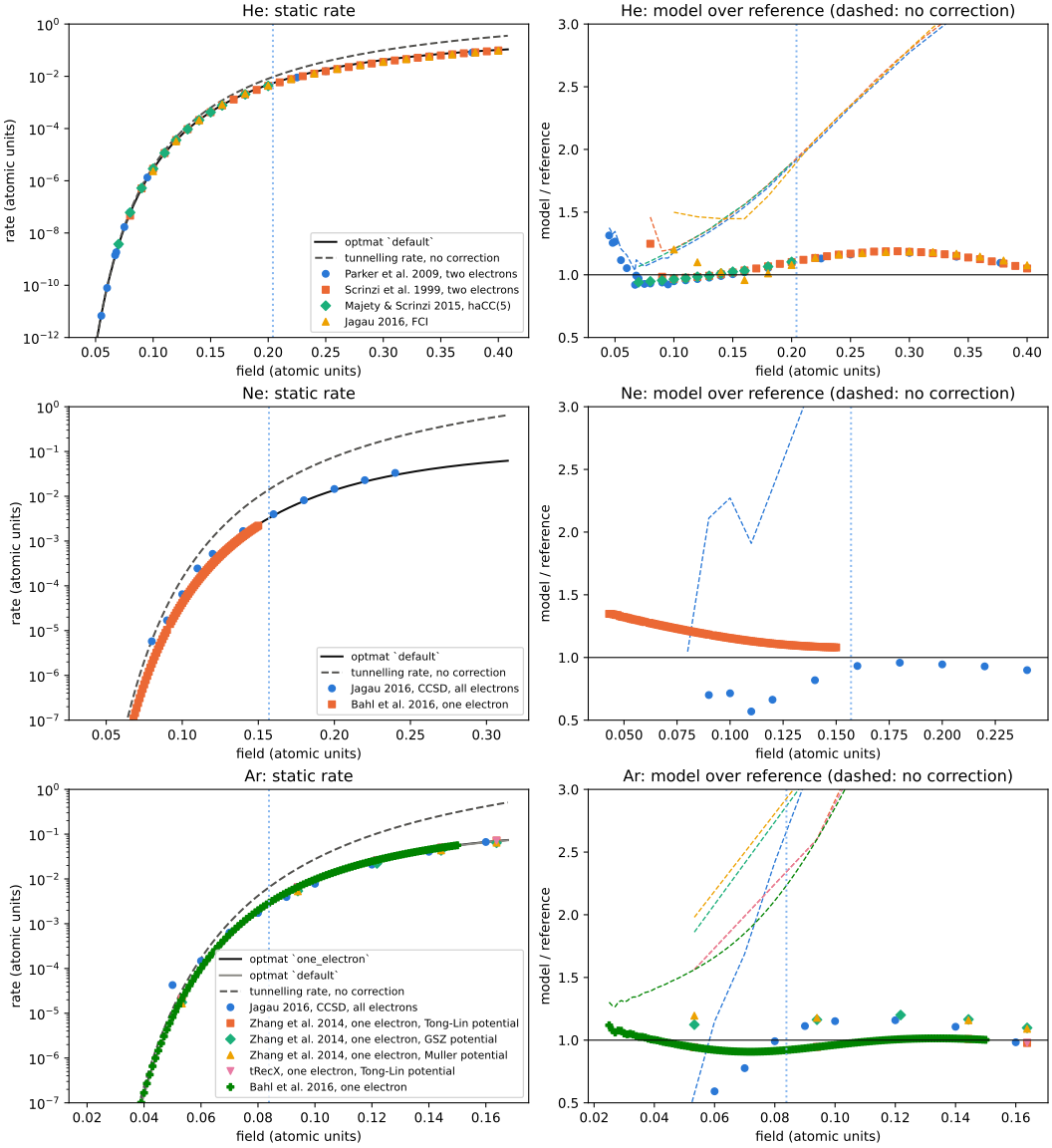
Ionisation: the static rates of helium, neon and argon

The static limit of the ionisation rate (optmat.gas.ionisation_rates) against the curated references (optmat.gas.ionisation_validation.static_rates()).

Helium (top): the rate of the atom, from integrations of the two-electron Schrödinger equation. The default model is the tunnelling rate of one electron with Tong and Lin’s correction, times an effective number of electrons of 1.47, which is the one constant set on these data (TC-658).

Neon (middle): the rate of the atom, from Jagau’s complex-scaled coupled-cluster calculation with all electrons correlated, against the default model, whose effective number of electrons is 1. Below 0.14 au the reference is not smooth in the field (TC-669).

Argon (bottom): the rate of one electron in a model potential, from Zhang, Lan and Lu’s exact solutions in three potentials, against the one_electron model (black), and the rate of the atom, from Jagau’s calculation, against the default model (grey), which differs from the former by the fine structure of the ion.

The right-hand panels are the ratio of model to reference. The dashed lines are the tunnelling rate without a correction (the static limit of the rate of Perelomov, Popov and Terent’ev, of Ammosov, Delone and Krainov, and of the forms of Ilkov et al. and Bergé et al.): it is too high at every field at which an atom ionises, by a factor of 2 already at six tenths of the barrier-suppression field \(F_b\) (dotted).

import math
import warnings

import matplotlib.pyplot as plt
import numpy as np
from _helpers import COLOURS, MARKERS

from optmat.constants import AU_ANGULAR_FREQUENCY, AU_FIELD
from optmat.exceptions import ModelRangeWarning
from optmat.gas.ionisation_rates import ionisation_rate_model
from optmat.gas.ionisation_validation import static_rates

fig, axes = plt.subplots(3, 2, figsize=(11, 12), layout="constrained")
ROWS = (("He", "default"), ("Ne", "default"), ("Ar", "one_electron"))
for row, (gas, name) in enumerate(ROWS):
    model = ionisation_rate_model(gas, math.inf, name)
    plain = ionisation_rate_model(gas, math.inf, "ppt_larochelle")
    barrier = model.barrier_suppression_field / AU_FIELD
    field = np.linspace(0.25, 2.0, 200) * barrier
    rate = model.instantaneous_rate(field * AU_FIELD) / AU_ANGULAR_FREQUENCY
    with warnings.catch_warnings():
        # Drawn beyond its range, to show how it fails.
        warnings.simplefilter("ignore", ModelRangeWarning)
        uncorrected = (
            plain.instantaneous_rate(field * AU_FIELD)
            * model.electrons
            / AU_ANGULAR_FREQUENCY
        )
    left, right = axes[row]
    left.semilogy(field, rate, color="#0b0b0b", label=f"optmat `{name}`")
    if name != "default":
        atom = ionisation_rate_model(gas, math.inf)
        left.semilogy(
            field,
            atom.instantaneous_rate(field * AU_FIELD) / AU_ANGULAR_FREQUENCY,
            color="#8a8984",
            label="optmat `default`",
        )
    left.semilogy(
        field,
        uncorrected,
        color="#52514e",
        ls="--",
        label="tunnelling rate, no correction",
    )
    for k, comparison in enumerate(static_rates(gas)):
        x = comparison.x / AU_FIELD
        style = {"color": COLOURS[k], "marker": MARKERS[k], "ls": "", "ms": 5}
        left.semilogy(x, comparison.expected, label=comparison.label, **style)
        right.plot(x, comparison.ratio, **style)
        with warnings.catch_warnings():
            warnings.simplefilter("ignore", ModelRangeWarning)
            without = (
                plain.instantaneous_rate(comparison.x)
                * model.electrons
                / AU_ANGULAR_FREQUENCY
            )
        right.plot(x, without / comparison.expected, color=COLOURS[k], ls="--", lw=1)
    for axis in (left, right):
        axis.axvline(barrier, color="#86b6ef", ls=":")
        axis.set_xlabel("field (atomic units)")
    right.axhline(1.0, color="#0b0b0b", lw=0.8)
    right.set_ylim(0.5, 3.0)
    left.set_ylim(1e-12 if gas == "He" else 1e-7, 1.0)
    left.set_ylabel("rate (atomic units)")
    right.set_ylabel("model / reference")
    left.set_title(f"{gas}: static rate")
    right.set_title(f"{gas}: model over reference (dashed: no correction)")
    left.legend(fontsize=8, loc="lower right")
plt.show()