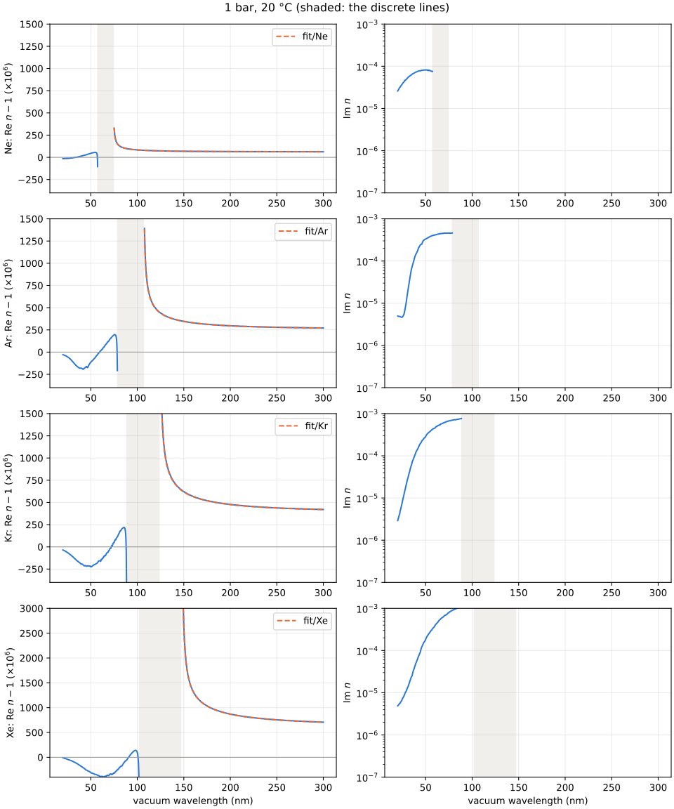
Neon, argon, krypton and xenon in the extreme ultraviolet

The complex refractive index at 1 bar and 20 °C, from 20 nm to beyond the first resonance, from each gas’s constrained oscillator-strength distribution (euv/Ne, euv/Ar, euv/Kr, euv/Xe): Chan et al.’s oscillator strengths, Henke’s scattering factors at high energy. Shaded: the region of the discrete lines, where the index is singular and the model carries no line widths. Dashed: the fitted model below the first resonance.

import matplotlib.pyplot as plt
import numpy as np

from optmat.conditions import State
from optmat.gas.euv import EV_PER_HARTREE, euv_model
from optmat.gas.models.fitted import fitted_models

state = State(1e5, 293.15)
fig, axes = plt.subplots(4, 2, figsize=(10, 12), layout="constrained")
for row, gas in enumerate(["Ne", "Ar", "Kr", "Xe"]):
    model = euv_model(gas)
    fit = fitted_models()[f"fit/{gas}"]
    threshold = 1239.84198e-9 / (model.distribution.threshold * EV_PER_HARTREE)
    first_line = 45.56335e-9 / model.distribution.line_energies[0]
    above = np.linspace(20e-9, threshold * 0.999, 400)
    below = np.linspace(first_line * 1.01, 300e-9, 300)
    for wavelength in (above, below):
        n = model.refractive_index(wavelength, state)
        axes[row, 0].plot(wavelength * 1e9, (n.real - 1) * 1e6, color="#2a78d6")
        axes[row, 1].semilogy(
            wavelength * 1e9, np.maximum(n.imag, 1e-12), color="#2a78d6"
        )
    axes[row, 0].plot(
        below * 1e9,
        fit.refractivity(below, state, warn=False) * 1e6,
        "--",
        color="#eb6834",
        label=f"fit/{gas}",
    )
    for axis in axes[row]:
        axis.axvspan(threshold * 1e9, first_line * 1e9, color="#f0efec", zorder=0)
        axis.grid(alpha=0.25)
    axes[row, 0].axhline(0, color="#9a9994", linewidth=0.8)
    axes[row, 0].set_ylabel(f"{gas}: Re $n - 1$ ($\\times 10^6$)")
    axes[row, 0].set_ylim(-400, 1500 if gas != "Xe" else 3000)
    axes[row, 0].legend()
    axes[row, 1].set_ylabel("Im $n$")
    axes[row, 1].set_ylim(1e-7, 1e-3)
axes[-1, 0].set_xlabel("vacuum wavelength (nm)")
axes[-1, 1].set_xlabel("vacuum wavelength (nm)")
fig.suptitle("1 bar, 20 °C (shaded: the discrete lines)")
plt.show()